How to Use Cell Coordinates and Range Codes in LibreOffice Calc

On LibreOffice Calc, there are various places, such as the "name box," where you must refer to a spreadsheet cell or to a range of cells (a rectangle of cells) using its strange code syntax, like A1:A1, A1:A2, A1:B2, A1:B2, A:A, $A1, A$1, $A$1, A:A~B:B, and so on. If you're familiar with Microsoft Excel, then perhaps it's not that strange. However, for me it's rather peculiar, specially since I had a lot of trouble finding its documentation. For reference, I'll write it down here.

What "A1" Means: Coordinate Codes

On LibreOffice Calc, every column is named after a letter, and every row is named after a number. Thus you have columns A, B, C, D, E, F, and rows 1, 2, 3, 4, 5, 6, and so on. To refer to a specific cell, we must combine both letter and number in this order.

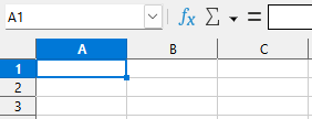
For example, the cell A1 is coordinates of the top-leftmost cell. It's always A1, in this order, column then row. It's not 1A. It's A1.

Observation: it seems these are officially called "cell references," which is impossible to find on Google if you don't know the name of it. I kept searching for "cell code" and all I got was documentation for programmers. I guess most people just don't call these things "code"?

$A$1: How to Stop Coordinates from Changing Automatically when Copying and Pasting

By default, cell coordinates are relative. This means if the coordinate is used in an expression in a cell and it's copied to a different cell, the coordinate will be automatically updated when you paste it.

For example, if you you 5 in the A1 cell, its value becomes 5 as a literal value. If you type =A1+10 in the B1 cell, the value of the B1 cell becomes an expression that is calculated based on the value of the A1 cell. In this case, 5+10=15, so the value you'll see on the B1 cell will be 15.

If you select the B1 cell by clicking on it with your mouse, copy it and paste it on B2, LibreOffice Calc will automatically change the expression to =A2+10. This means that if you keep copying and pasting the same cell downwards the column, the expression will always refer to the cell on its left side, which is normally what you want when you're working with spreadsheets. If this was a cell to calculate the total or SUM of the cells to the left, you could just copy and paste it through the entire spreadsheet and it would work.

However, in some cases you don't want this to happen. For example, if cell A1 has a special value that you want to refer to in all your expressions that you just happened to place in that cell specifically, you wouldn't want it to change automatically when copying and pasting things.

In this case you can use the dollar sign ($) to tell LibreOffice Calc that it shouldn't update the coordinate automatically.

This dollar sign can be placed before the column code and before the row code.

$A1 means that A never changes, but 1 may change, i.e. it's always the same column, but the row is allowed to change.

A$1 means that A may change, but 1 never changes, i.e. it's always the same row, but the column is allowed to change.

$A$1 means that it's always the same cell.

Important: if you use $A$1 and you cut and paste the A1 cell to somewhere else, e.g. to A2, then LibreOffice Calc will automatically update all references to $A$1 changing them to $A$2. This means if you want to keep them referring to A1 you shouldn't cut and paste it, but instead copy and paste first and then delete A1 or change it to a new value.

Observation: the LibreOffice Calc guide book calls coordinates like A1 relative references and coordinates like $A$1 absolute references.

Selecting Rectangles

In many places where a function may apply to several cells you're supposed to use a special code for a cell range, which means that to select or to specify cells we must specify a range that starts at one cell and ends at another cell. These two coordinates are separated by a colon (:).

For example, A1:B2 is a rectangle from the first column (A), first row (1), to the second column (B), second row (2).

If both coordinates have the same number, then it's a single-row rectangle, a horizontal rectangle. For example, A1:B1 selects the first two cells of the first row.

If both coordinates have the same letter, then it's a single-column rectangle, a vertical rectangle. For example, A1:A2 selects the first two cells of the first column.

Selecting a Single Cell with a Range

To select a single cell with a range, simply make the range start and end at the same cell.

For example, to select A1, the range is A1:A1. A rectangle that starts at A1 and ends at A1.

Selecting a Whole Column

To select a whole column, the code is the column letter, a colon, and the column letter again. For example, A:A selects the whole A column.

Selecting Multiple Whole Columns

To select multiple whole columns, the code is the starting column letter, a colon, and the ending column letter. For example, A:B selects the columns A and B, while A:C selects A, B, and C.

Selecting a Whole Row

Similarly, to select a whole row the code is 1:1 for the row 1, 2:2 for the row 2 and so on.

Selecting Multiple Whole Rows

Likewise, to select multiple whole rows the code is 1:2 for rows 1 and 2, 1:3 for rows 1, 2, and 3, and so on.

Combining Separate Rectangles

It's possible to select multiple rectangles at once through the concatenating operator, which is a tilde (~).

For example, A:A~C:C selects both A and C columns entirely, but skips the B column.

Selecting Cells from Other Sheets

On LibreOffice Calc we can have multiple sheets in a single document by adding them in the sheet bar above the statusbar. It's possible to refer to a cell that is in a different sheet. This is useful if you want to separate the main data you're working on from special values that you would keep in a different sheet just for them.

To reference a sheet that doesn't have spaces in its name, type a dollar sign ($), its name, a dot (.), and then the cell coordinates.

For example, $Sheet2.$A$1:$A$3 selects a tall rectangle from the sheet called Sheet2.

Important: the rules about coordinates apply to cross-sheet references too! Think of sheets as a third dimension. Column is the first axis, row the second axis, and sheet the third axis. If you refer to Sheet2.A1:A3 on a sheet's A1 cell, and then copy paste it to B1, the coordinates will be automatically updated to Sheet2.B1:B3. This means, for example, that you could put cells to calculate the totals of one sheet on a separate sheet, and when you add a new column to the first sheet you simply copy and paste a cell on the second sheet. To prevent this from happening we need the dollar sign ($).

Important: if we don't use a dollar sign before the name of the sheet being referenced and we duplicate the sheet that is referencing it, Calc will change the sheet being referenced according to the order of the sheets on the sheet bar. For example, if we have the sheets Apple, Banana, and Coconut, and we refer to Apple from Coconut, and then we duplicate Coconut, the newly created sheet Coconut 2 will refer to Banana instead of Apple. That's because Coconut is the 3rd sheet referencing the 1st sheet. Since Coconut 2 will be the 4th sheet created just to the right of Coconut, it will refer to the 2nd sheet. It's kind of confusing that it works like this, but it's at least consistent.

Selecting Sheets with Spaces in Their Names

If the sheet has spaces in its name, we must enclose the name with single quotes (') so that LibreOffice Calc knows where the name starts and ends.

For example, $'Personal Budget'.A:A selects the A column from a sheet called "Personal Budget."

Selecting Sheets with Quotes in Their Names

If a sheet's name has a single quote (') character in it, we must escape it in order to refer to it. Normally, we would use \' to escape things like this, but this doesn't work on LibreOffice Calc. Instead, single quotes are escape with another single quote, like this: ''.

For example, if our spreadsheet is called Santa's Sheet, we must type $'Santa''s Sheet'.A:A to select the A column.

Important: LibreOffice Calc will update sheets' references automatically if you rename a sheet. This means that if you don't know how to refer to a sheet, or you forgot how to escape a character, you can simply rename the sheet to Sheet2 or something simple like that, refer to it in an expression, then rename it back to what it was before, and Calc will automatically update the code you used adding quotes and properly escaping everything that needs to be escape.

Cuboid Selection

It's possible to use a 3D range across spreadsheets. I have no idea why would you ever want to do that, but it's possible. To do this, you must make sure that your spreadsheets are in the right order you want in the spreadsheet bar, and simply use the syntax we have already learned about.

For example, let's say we have the spreadsheets January, February, March, April, and so on. One for each month, and in the correct order.

We could use $January.A:$March.F to select all the cells from the columns A:F (A to F) of all the spreadsheets from January to March.

Selecting a Whole Spreadsheet

I haven't been able to figure out if there is a specific code for selecting an entire sheet, so I think you'll need to specify either a column range or a row range for this, like $Sheet2.A:Z.

Observation: if you click on the top-left rectangle on the sheet's border, the range A1:XFD1048576 will appear in the name box. This is the maximum amount of rows and columns that Calc supports. Unfortunately, it doesn't tell us whether there is a code for this or not. If you click on the column name for the A column on this border, it will select the whole column, but won't display A:A on the name box. Instead, it displays A1:A1048576 because Calc supports a maximum of 1048576 rows.

Intersecting Selections

It's possible to specify a range that is an intersection of two other ranges using an exclamation mark (!).

For example, A:C!B:D is the same thing as B:C.

With code this is rather useless, but there is an option called "Automatically find column and row labels" in Tools > Options > LibreOffice Calc > Calculate that is disabled by default, but when enabled allows you to type names of columns and rows instead of letters and numbers.

An example given by the LibreOffice Calc guide book is that if you have columns labelled January, February and so on, and one of the rows is labelled Temperature, you can refer to the cell of a given month in the Temperature row by writing a code like this:

'February' ! 'Temperature'

Literally this would be the intersection of all cells in the February column with all cells in the Temperature row, but because it's an intersection of one row with one column, the result is just the cell of that row in that column.

Using Named Ranges

It's possible to give a name to a range so you can refer to it in expressions and manage it all in one place. To do this, follow the following steps:

1: click on Sheet -> Named Ranges and Expressions -> Define... on the menubar. A dialog window will appear for you to create a new range.

2: give it a name like My_Subtotals. The name may not include space characters.

3: type the cell code for the range, or simply click and drag on the sheet to select it.

4: press the Add button to add it.

To use it in an expression, simply type its name. For example:

=SUM(My_Subtotals)

Although you don't need to name your variables prefixing them with My_, personally I think it's a good idea, specially if you don't use spreadsheets a lot. That's because if you revisit your spreadsheet in a few weeks, or a few months, you may not remember what part of the code comes from Calc's standard library and what part of the code comes from your own custom definitions, variables, functions, and named ranges, so it's a good idea to make this clear in the name to save your future self the trouble of trying to figure out what the code means.

Selecting Cells using Cell Codes in Strings or Other Cells

In some peculiar cases you may want to select a cell whose coordinates are specified in another cell. Indirection is one of programming's greatest wonders, so it makes me happy that LibreOffice Calc provides a way to do this through the INDIRECT function¹.

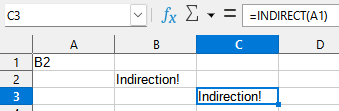
=INDIRECT("A1")

The code above has the string literal "A1". It does the same thing as just typing A1, so it's not very useful. What is useful is if we do this:

=INDIRECT(A1)

Now Calc will resolve the value of A1, turning it into a string. For example, if the cell A1 has B2 written on it, then A1 will be replaced by the string literal "B2".

=INDIRECT("B2")

And this is the same thing as just typing B2.

If you ever wonder how pointers work in programming, this is how they work in programming. In fact, if anyone asks me how they work, I'm just going to show them this article. It explains everything.

It's also possible to concatenate strings using & in Calc, so you could have something like this:

=INDIRECT("B" & A1)

Now if A1 has just the number 2 written on it, the concatenation above will result in "B2", and that's what will be passed to the INDIRECT function. Or you could have the column letter and the row number in different cells, and use A1 & B1 for example to concatenate them.

Documentation

• https://help.libreoffice.org/latest/en-US/text/scalc/guide/relativ_absolut_ref.html (accessed 2025-02-07)
• https://books.libreoffice.org/en/CG24/CG2408-FormulasAndFunctions.html#toc16 (accessed 2025-02-07)
• https://help.libreoffice.org/latest/en-US/text/scalc/01/04060109.html?DbPAR=CALC#bm_id3153181 (accessed 2025-02-07)

References

1. https://ask.libreoffice.org/t/how-to-reference-a-cell-using-a-formula/57344/4 (accessed 2025-02-07) ↩︎